
[Note: this is a somewhat technical / mathematical article, so those of you who only want the daily Corona updates, “the current numbers”, might want to skip this one]
As we all probably know by now, the official numbers on number of infected (‘Confirmed’) are not correct – they can’t be correct because that would require that we would test everybody, which clearly is impossible. So we know that the official numbers on confirmed and mortality rate are off, but by how much…?
So, there’s also uncertainty about the true mortality rate, initially estimated at 2-5 %, based on the known confirmed cases, and with a current global mean value of 3%.
But since many countries now test only those in critical condition, and official mortality rates ranging up to almost 10% in some countries, there’s reason to believe that the actual mortality rate is lower than expected, perhaps much lower.
Yesterday I linked to an article by Stanford Professor Ioannidis, where he argues the same, i.e. that the current estimates on mortality are way too high, and uses data from the cruise ship Diamond Princess (which can be regarded as a controlled experiment, since everybody onboard were tested) to infer that the true mortality rate most likely resides in the range 0.025% to 0.625%, that is, way below the current estimates, and way below what the official numbers show. Note that the data from Diamond Princess are very thin, only 700 infected data points and 7 deceased, so there’s quite a bit of uncertainty because a fairly limited sample size.
So, given that the official mortality rate estimate, based on the number of known confirmed cases is wrong, how can we go about estimating the true number ? And since the current testing practices in many countries now solely focus on the critical cases, meaning that there’s probably lots of unknown cases flying under the radar, how can we estimate the true number of infected…?
One way could be to use the following equation for an estimate:
D = C x F x R
(note: the R in the equation above has nothing to do with the R0-value mentioned in any scientific article about spread of virus!)
where D stands for number of deceased, C for the number of known, confirmed cases, F for factor to multiply the known confirmed cases to get the true number of infected, and R for the mortality rate.
However, the problem is that we don’t know F nor R, the only variable in the equation that we do know, is C, the number of confirmed cases. So, we can’t solve that equation analytically.
But, we could use the equation above, simulating (lot’s of!) unknown F’s and unknown R’s, and use the known C, to simulate the number of dead per day, and then for each combination of R and F, compare that generated number to the actual number of deceased for that day.
That is, we can use brute force, i.e. numerical methods on our computer, to estimate the parameters.
One way to do that would be by grid approximation, i.e to discretize the parameter space, that is, basically creating (in this case) a two-dimensional matrix with millions of combinations of possible parameter combinations, and see what each of those parameter combinations generate in terms of simulated deaths.
I did just that yesterday for a number of countries, and below the resulting M and F values for a few selected countries:
                R               F
COUNTRY

China          1.0%             4
US             1.2%             1
Italy          4.5%             2
Spain          1.7%             3.5
S. Korea       0.7%             1.5
So we can see that except for Italy, the estimated mortality rate obtained by this method is about 1%, which is quite a bit below the “official” 2-5%.
However, by using this method, we only get a single number for each of the params, we don’t get any indication on the level of uncertainty in the estimates.
So, instead of using grid approximation, let’s use the BIG HAMMER, Markov Chain Monte Carlo, a method originating from the Manhattan Project @ Los Alamos, with guys like Robert Oppenheimer, Stanislav Ulam, John von Neumann, Nicholas Metropolis and others.
So, let’s use the Big Hammer, and see what we get. I’m using Python, Pandas and in particular, PYMC for the Bayesian inference, that is, PYMC does, using MCMC, all the “counting” to figure out the most likely values for the parameters R and F, given the data that we’ve actually seen, that is, the number of confirmed and the number of “true” deaths.
Now, a huge benefit of Bayesian methods that we get the full probability distribution, not just a single point number, for the parameters we want to estimate, that is, R and F. Therefore, I’ll present the results from the MCMC-runs as histograms, showing the probability distribution for each parameter:
Results of Baysian Inference
Diamond Princess:
Let’s start by looking at the only known “Controlled Experiment”, the cruise ship Diamond Princess, as mentioned in the article by John Ioannidis above:
Professor Ioannidis found, in his calculations, that the true mortality rate, based on this “controlled experiment”, most likely resides in the range of 0.025% – 0.625%.
Let’s see what my engine thinks:
It finds a fairly symmetrical distribution for R, with a peak at 0.25%, well within the range given by Professor Ioannidis.

China
China, using MCMC: we can see that the R parameter peaks at 1.2%, (official mortality rate 4%) but that most of the probability density resides below that value. (Unfortunately I forgot to add code to show Credible Intervals in these graphs, and since each run takes about an hour, I’m not going to run them again). For parameter F, the inference engine finds the peak just under a factor of 3, with most density above that value.

Italy
Italy: R peaks somewhere between 2.5 – 2.75%, and F peaks around 3, with most density above that value. There’s a huge difference between the “official” mortality rate of 9%, vs. what my inference engine comes up with!

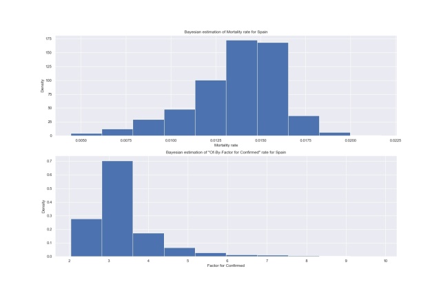
Spain
Spain: R peaks around 1.5%, F around 3. Again, the official R value for Spain is 6%, my inference enging thinks it’s about 1.5%.
Japan
Japan: R peaks at 1 %, F at 3. Official R for Japan is 3.7%.

South Korea
South Korea R peaks at 0.3%, F at 3. Official R value is 1.2

United States
US: R peaks at 0.5%, F at 3. Official R value for US is 1.3

Sweden
Sweden: R peak at 0.3%, F at 3. Official R-value at 1.1%

Global inference results
Consolidating all countries into a global result, we get R peak at about 1.2%, with most of the density below that peak. And we get F peaking at a bit below factor 3.

Conclusion
So, from all examples above, we can see that my Bayesian Inference Engine estimates that the true mortality rate R is 1% or less for most countries, a factor 3 less than what’s given by the official numbers. The same goes also at the global level.
And if that’s true, that is, the mortality rate is 1% or even below, that is very very good news for all of us, since that means that a factor 3 fewer people than currently estimated will die from the virus.


