
A few days ago, I did a quick & dirty Bayesian estimate on Covid Vaccine Efficacy, based on Israeli data, given in a Twitter post (see details on the data in the link above).
As stated in the earlier post, there are several caveats with that analysis, the most fundamental two are:
- Since I don’t know Hebrew, I’ve not been able to verify the data and its source (although the Twitter post does reference the source (health.gov.il). So, in what follows, I’m assuming that the numbers as given in the Twitter post are accurate.
- The given data is only for the period of June 27:th to July 3:d, meaning that we have very little data to work with, covering only a very short period. Thus, even when assuming the given numbers are accurate, there’s a lot of uncertainty in any estimates based on that small amount of data, and the short period. How much uncertainty…? It is exactly in this type of situation – a limited amount of data – that Bayesian Inference, providing not only point estimates (combined with p-values that I’ve never really understood), but full probability distributions, can help us get a handle on what that uncertainty looks like, how much uncertainty there is.
The model I’m using in this analysis is a bit more complex than the previous one : the current model is hierarchical, using partial pooling of vax status & age group based data, the idea being that regardless of age, there is _some_ commonality between the age groups in terms of vaccine efficacy. The result of this is something called “shrinkage“, where the individual age group based estimates are “pulled” a bit towards the overall mean parameter value.
Warm-Up by a quick look first at the Pfizer Trial Vaccine Efficacy Data
(For those of you not very interested in the technicalities of Bayesian analysis, feel free to skip this section and jump straight to the section on Israeli data below)
First, let’s apply a very simple Bayesian model (*fully* pooled, like standard A/B-testing) to the Pfizer trial data, from this Lancet article, the one where I believe the 95% Efficacy numbers originate from:
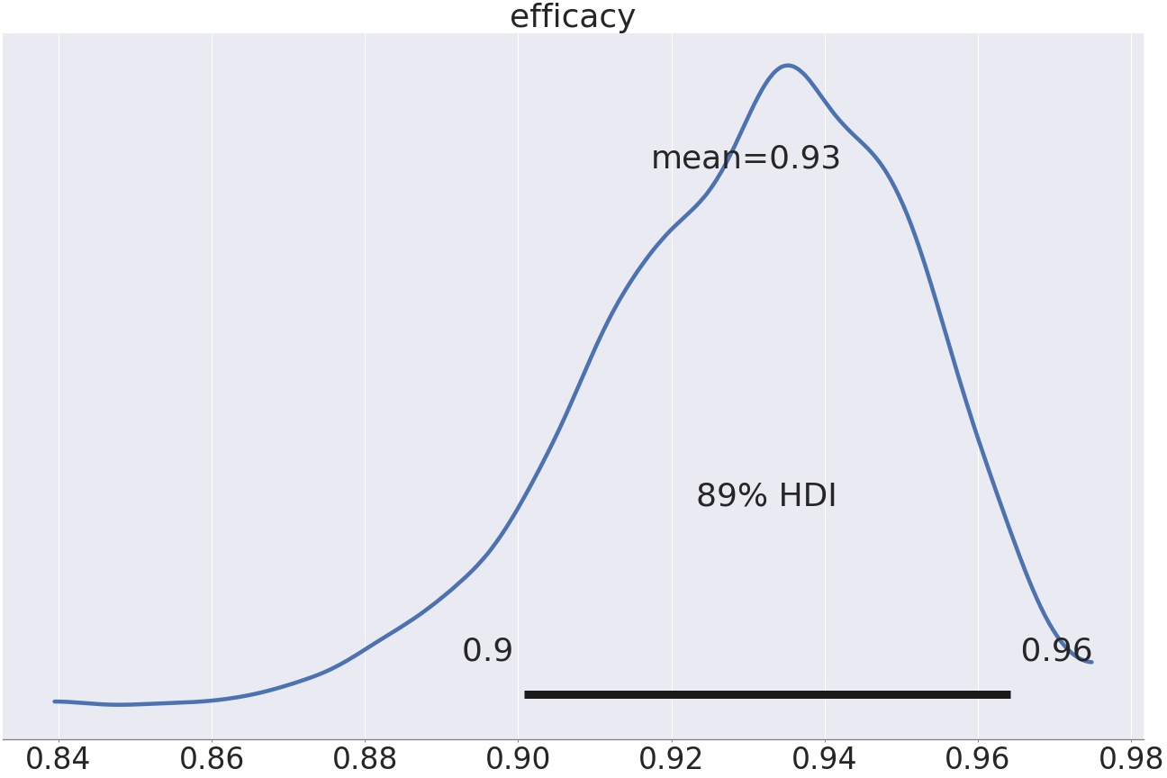
My simplistic model reports an Efficacy rate of 93%, with a 89% credible interval ranging from 0.90 to 0.96. That is, very close to the numbers reported in the official trial data.
We can also run a partially pooled model on the Pfizer data for comparison. Basically, the difference is that in the partially pooled model below, the two incidence rates, test group vs control group, are not *fully* independent, instead they experience “shrinkage“, that is, a bit of ‘pull’ from each other, the less data, the more pull. Both incidence rates are therefore pulled down a bit, the group with less data pulled proportionally more.
The canonical analogy (credit to Richard McElreath) for explaining how partially pooled models work is as follows:
Imagine you are a Martian on your first visit to Earth, and you are interested in waiting times at cafe’s. Before your first visit, you have absolutely no idea on how long you’d typically have to wait for your cuppa, so your expectation on the waiting time covers a huge range. Let’s say you visit your first café in Stockholm, and you have to wait 5 min. Now, you have a bit more information on what the average waiting time might be. So you update your prior. Next, you visit a few more cafés in Stockholm, and by Bayesian updating, arrive at an expected waiting time of 3 min. Next, you travel to Oslo, and study café waiting times there. The question is: should you now reset your expectation to your initial, wide one (since you have no a priori info on the waiting times in cafés in Oslo (your experience is exclusively from Stockholm) ? That is, should you forget all about what you learned about cafe waiting times in Stockholm, now that you are in Oslo ? That is, are you subject to retrograde amnesia all of sudden, because you moved from Stockholm to Oslo ?
If you believe that the waiting times in Stockholm vs Oslo are totally independent, i.e. there’s no value in knowing the avg. waiting time in Stockholm when you are in Oslo, then, you should pool your model fully, that is, treat Oslo cafés as a totally different species than Stockholm cafés. On the other hand, if you believe that waiting times in Starbuck’s Stockholm and Starbuck’s Oslo probably are not that dissimilar, then you want to model the waiting time as a partially pooled one, that is, using some of what you learned in Stockholm when studying Oslo, that is, the data from Stockholm has some influence on your Oslo prediction.
So, below the Pfizer data modeled with a partial pooling model:

Using the partial pooling model, the efficacy is a smitheren higher, 94% instead of 93.
We can see the shrinkage clearly by looking at the descriptive stats for the two models (fully pooled vs. partially pooled):

The above table shows the two models, “Full Pool” vs “Partial Pool”, and three desc.stats for each: mean, HDI low, HDI high (for a 89% Credible interval). We have two parameters of interest: alpha[0], which is the incidence rate for the control group (non-vaccinated), and alpha[1] which is the incidence rate for the test group (vaccinated). These params are on a log-odds scale.
The two p_alpha parameters are derived from the log-odds alphas, and show the incidence on a normal 0-1 probability scale for the two cohorts. Efficacy is on normal probability scale, and the parameter of our main interest. Finally, alpha_bar is the log-odds hyperparam for alpha. alpha_bar makes the model hierarchical, partially pooled and enables shrinkage, and p_alpha_bar is its representation on a normal probability scale.
If we focus on the two p_alphas, we can see that both of them gets a tiny bit smaller when going from fully pooled to partially pooled model. That is, both of them is pulled towards a common mean (p_alpha_bar). This is shrinkage in action, enabled by the hyperparam alpha_bar, a common “ancestor” to both alphas.
Finally, for this rather technical section, we can take a look at a forest plot showing the difference between the fully pooled (red) and partially-pooled (orange) models :

For a good intro to hierachical models, pooling and shrinkage, take a look at this blog post.
Now, let’s look at the Israeli data:
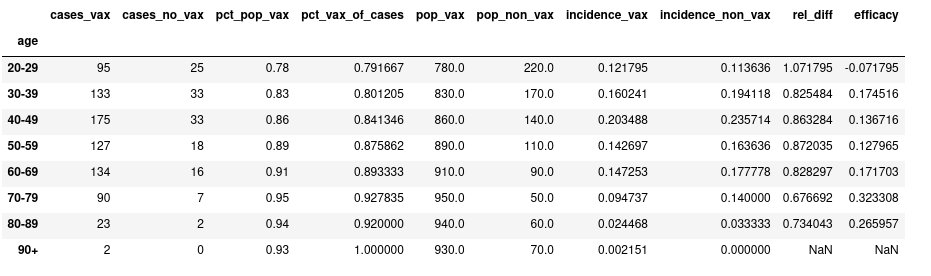
For reference, here’s a dataframe with the data from that Twitter post, combined with point estimates on incidence and efficacy (assuming a population size for each age group) :
Let’s next run the new, hierarchical model on this data, and first look at the distributions for incidence rates, non-vaxed (green) vs vaxed (red):

A couple of observations to make:
- notice that the credible intervals (~~confidence intervals for the Frequentists among us 🙂 are much wider for the non-vaccinated vs the vaccinated. Why…? Because there’s much more data on the vaccinated, since most Israelis are now vaccinated, thus the model is more certain on the vaccinated.
- notice that for the cohort with the least amount of data, the non-vaxed 80-89 year olds, the incidence rate (as given by the round marker) has been pulled up from it’s calculated value 0.03 from the dataframe above, to 0.07. Shrinkage in action!
Next, lets look at the Vaccine Efficacy distributions, per age group:
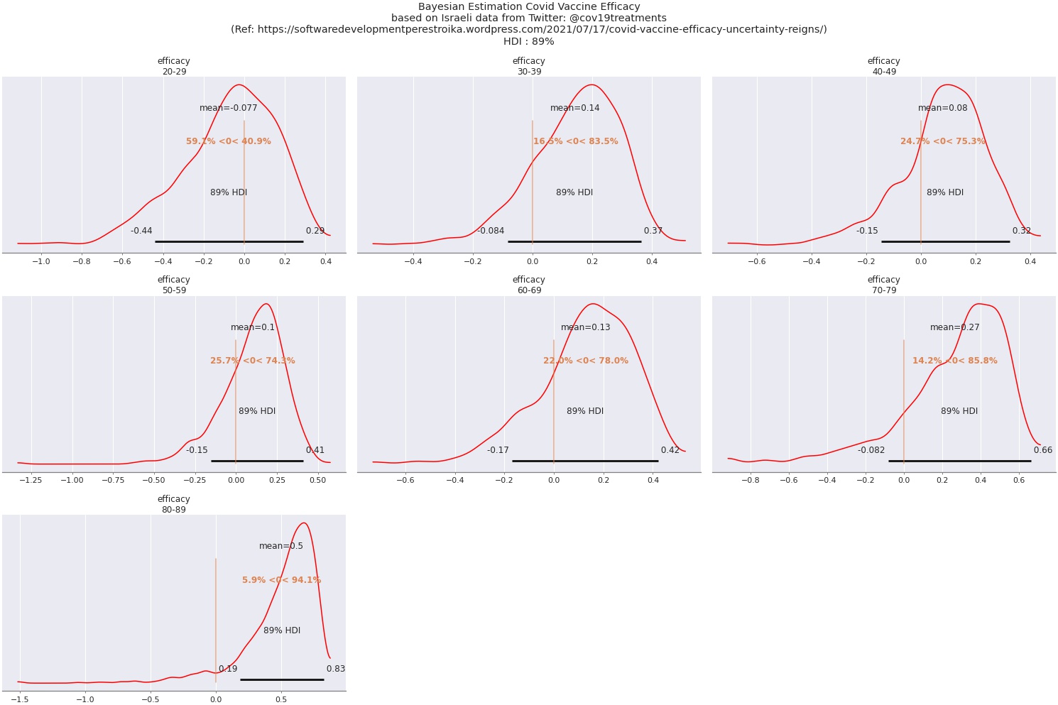
Again, a couple of things to notice:
- Vaccine Efficacy calculated on this (very limited!) data is far from the 95% of the pre-release trials.
- The uncertainty is huge: the credible interval for all age groups except 80-89 spans over zero
- Age group 80-89 has been pulled upwards by shrinkage quite a lot. With the very low calculated incidence rates for this group, combined with shrinkage, that is, the non-vax incidence rate being pulled up from 0.03 to 0.07 (which is still way lower than the rates for the rest of the npn-vax groups), Efficacy for this group ends up at about 50%, however, with a wide credible interval.
We can also look at a forest plot of the same data:

Summary
So, what conclusions regarding Vaccine Efficacy would I draw from this analysis…?
The short answer is: almost none. First, because I don’t have a clue regarding the quality of the data. Secondly, because there’s very little data. And thirdly, because the analysis makes it clear that there’s a lot of uncertainty in the results. But that last point is actually a valuable finding : I’ve seen a lot of Twitter posts referencing this dataset and drawing full blown conclusions from it, but with a bit of Bayesian analysis, we can now appreciate that before jumping to any conclusions, we need more data, and we need to confirm data quality.


